

Global and Local Explainability of Graph Neural Network Chemistry
GNNs do not learn features. They learn the rules for creating them, and through repeated message passing those rules sculpt a latent space that is rich enough to predict many chemical properties at once.
How can graph neural networks learn a complex quantum chemical solutions simply by training on molecular graphs? The key lies in their ability to build their own representation rather than relying on pre engineered descriptors. GNN learns the rules for creating the features that best support accurate prediction. This happens through message passing, the core mechanism by which each atom iteratively updates its state using information from its neighbors.
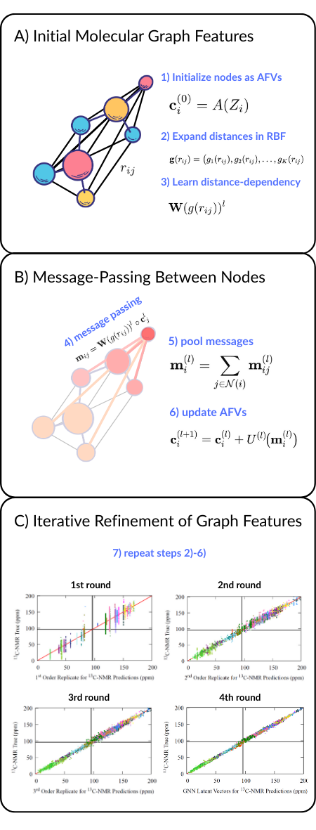
Message passing GNNs can be understood in seven broad steps. For full architectural detail and mathematical definition, see the previous post. Here we focus on the conceptual flow.
Steps 1 - 3 - Initializing the molecular graph nodes/edges
Raw atomic numbers are expanded into an atom feature vector (AFV) space of user-chosen size (128-D). Size is directly controlling width of the GNN’s feature representation (width of neural net)
Raw internuclear distances are expanded using a radial basis set of functions. Expansions is necessary to match width of features required by GNN algorithms
Distance dependency is tuned based on learned dense neural network design which reduces RBF dimensionality to the same width of the AFV (128-D)
Steps 4-6 - Message-passing updates
Message-passing step where learned distance dependency times modulated by the neighboring nodes updates each AFV
Messages from all neighbors are pooled
Update network learns how messages should update initial AFV
Step 7 - Repeat steps 2-6 - Iterative repeats refine prediction
The objective of this post is to illustrate how message passing works by using a simplified proxy model capable of replicating the AFV space produced by the full GNN pass. With a minimal formulation of graph message passing, we show that the essential structure of the AFV space can be reconstructed, which demonstrates that the core mechanism driving GNN representations is the iterative exchange of local information rather than the full architectural complexity.
Fig 1 - Seven broad steps to a message-passing GNN. Repetition of these steps results in finer predictions.
The proxy framework that will be introduced lets us examine message passing step by step, revealing how each iteration refines atomic features and progressively improves property predictions.. Crucially, the AFV space has already been demonstrated as a transferable representation for downstream property prediction, see previous post, we use transfer learning examples here to emphasize that this mechanism is not specific to a single task but reflects the general representational capacity of message passing itself. Thus the results we present apply to any property that can be learned from the AFV space and not only the GNN. Typically, We find that only a small number of refinements, typically fewer than four, are needed for the representation to converge, reflecting the inherently local nature of chemical environments and how information propagates from node to node.
We can evaluate our global AFV reconstruction quantitatively by comparing the reconstructed atom vectors to the original GNN AFVs as the number of refinement steps M increases. Table 1 reports this accuracy and also introduces the notion of neighborhood depth, which specifies how far information is allowed to propagate in each update. Depth equal to 1 corresponds to using only direct neighbors, while larger depths include atoms several bonds away. Increasing the depth expands the effective chemical neighborhood available to each update and significantly improves reconstruction quality, especially for long range correlations, as confirmed by the results.

To replicate the AFV space we use supervised learning directly on the full GNN pass AFV space, but the features supplied to our model arise from a deliberately simplified message passing framework. This framework uses a minimal update rule applied to each atom and its neighbors, allowing us to isolate the core mechanism by which GNNs build their representations. The goal is to demonstrate that the AFV space is reconstructable through message passing, regardless of initial representation used.
By reducing the full GNN architecture to its essential iterative update structure, we obtain a model that is both easier to interpret and broadly explanatory across all downstream domains where transfer learning from the AFV space is effective.
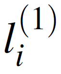
The supervised learning scheme is based on fitting the equation below to the full pass GNN AFV space, repeated in successive message-passing rounds. The first round defined as:


A Simpler Framework For Message Passing Reconstructs AFV
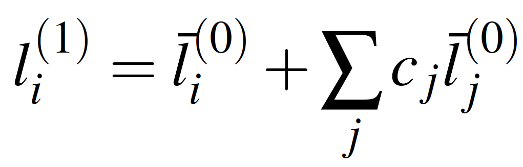
The starting point atom vector (random initial guess fixed for each Z)
Neighbor j’s starting point vector (random initial guess fixed for each Z).
Weighting coefficients that will determine the effect neighbor j has on target atom i. This will be fitted with data (supervised learning)
Our atom vector updated based on the identity of our initial neighboring vectors
With the first update complete, we repeat the procedure, fitting again to the AFV space but now using the outputs of the initial message passing iteration as input. After this first pass, each atom has been adjusted based on its immediate neighbors, meaning that what began as a random neighbor vector is now informed by that neighbor’s own environment. A second application of the same update rule refines the AFVs again, this time incorporating information from neighbors of neighbors. In general, the Mth update is computed from the neighborhoods defined at step M - 1, so after M refinements each atom has effectively received information propagated from all atoms within depth M of the molecular graph.

In this way the AFV space can be reconstructed through a simple repeated operation calibrated to the true GNN outputs. Later we show how this reconstruction mechanism accounts for the accuracy of GNN predictions with transfer learning examples to highlight the versatility of the AFV representation itself in modelling chemical properties, no longer needing the full GNN pass.
There is an additional subtlety in how neighborhoods are defined at each step. At every update we may choose to aggregate information only from direct neighbors, which is computationally efficient, or we may explicitly include information from second neighbors, third neighbors, or larger local regions. Both approaches converge to a similar AFV representation. The difference is how quickly information from more distant atoms becomes available to a given node and that some complex many-body information may be lost but as we will show this is considerably very small. Nevertheless, if only direct neighbors are used at each update, then the representation must be refined more times before distant atoms influence the updated AFV.
Reconstructing the AFV Space with Simple Message-Passing Framework and Effect on Transfer Learning
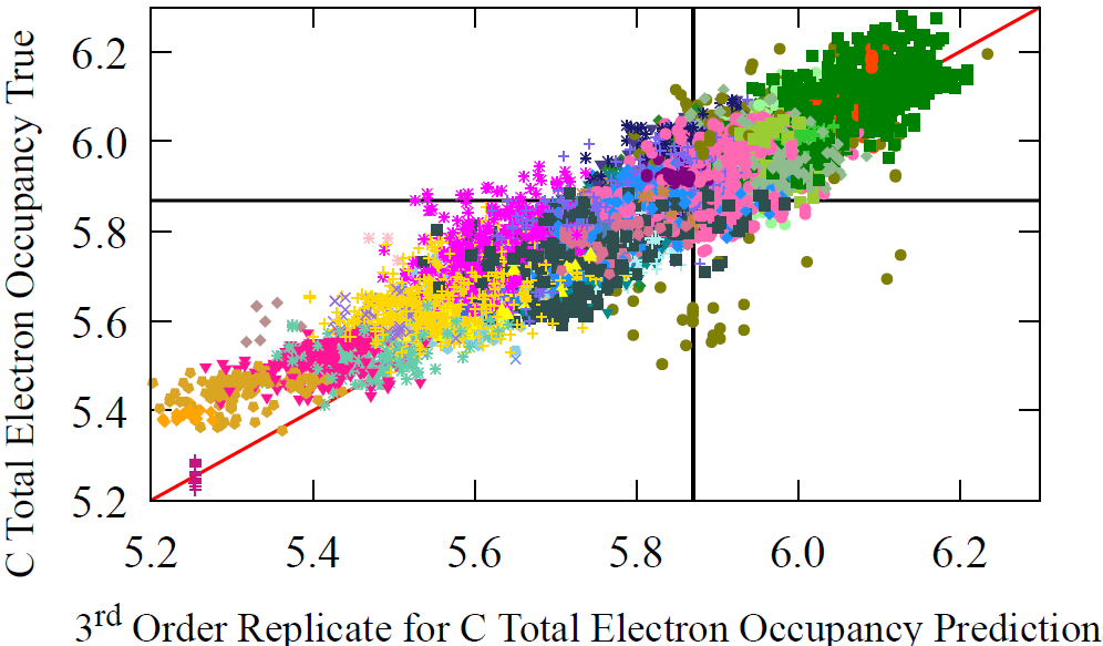
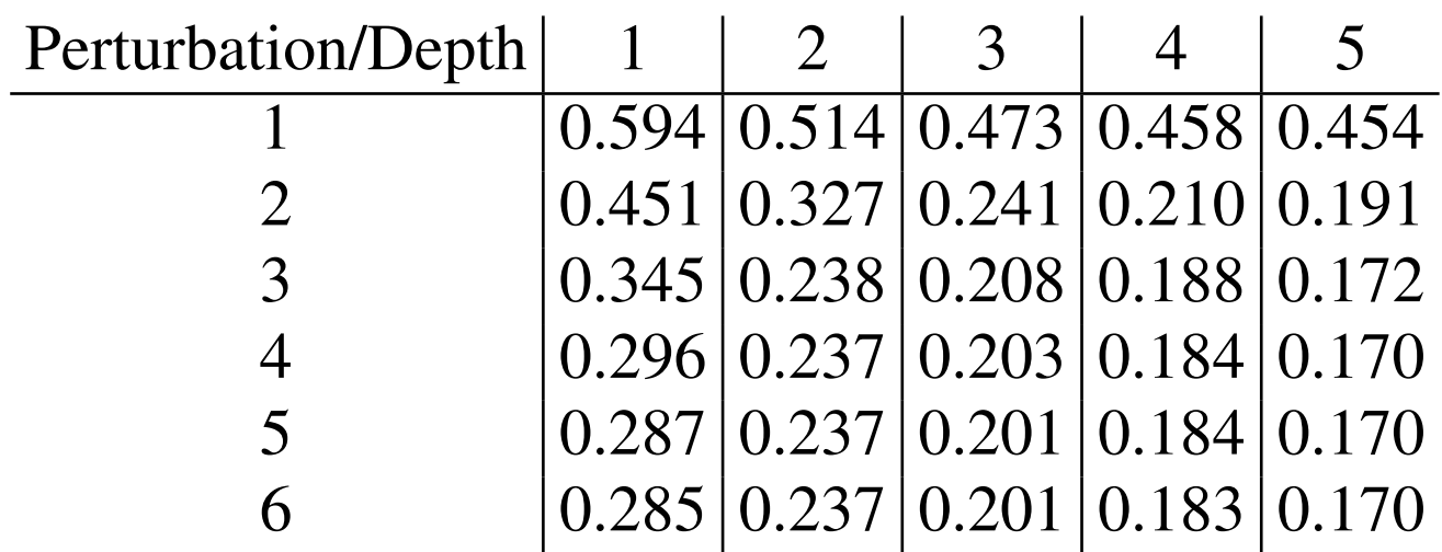
Table 1 - root mean square error (RMSE) of our reconstructed AFVs vs. the GNN AFVs, over several iterations of our self-consistent scheme (down), and with increasing neighborhood depth (across).
For any depth smaller than the total molecular diameter, some many body information is necessarily excluded, meaning that even with arbitrarily many refinements the reconstruction cannot fully match the accuracy achieved at larger depths. In practice, however, this loss is negligible. The average magnitude of an atom feature vector is roughly 12.8 units, so the residual error introduced by limiting the neighborhood remains small relative to the overall scale of the AFVs.
The iterative reconstruction of the AFV space should have direct consequences for the downstream properties predicted from this representation. This includes the original target of the GNN, such as total energy, but also any properties learned through transfer learning, as discussed in a previous post. If the AFV space captures the essential chemical information needed for these tasks, then improving its reconstruction should improve the accuracy of both the primary prediction and the transfer learned models. In this sense, the AFV representation functions as a fundamental framework for evaluating how message passing shapes predictive performance across a wide range of molecular properties.
Below we have the predictions for C-NMR using the reconstructed AFVs over four updates with a neighborhood depth of one. For the transfer model’s forward pass used for NMR, see previous post on transfer learning from pretrained AFVs.
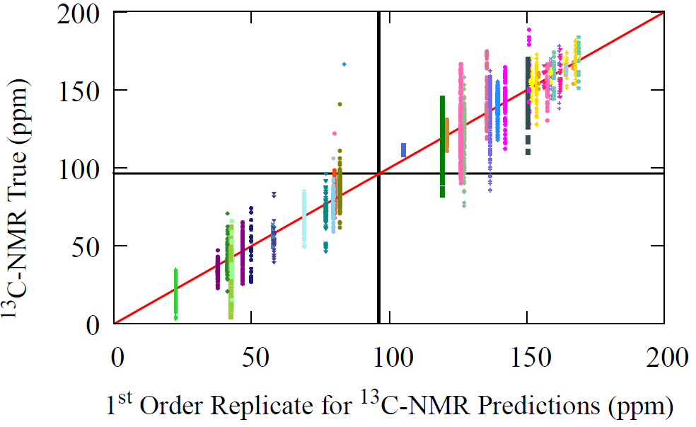
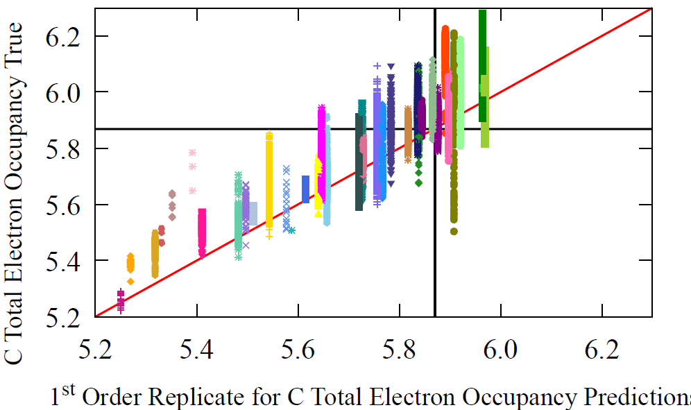


Fig 6 - The performance of our reconstructed AFV space with message passing, over successive refinements (M) of the procedure. The zeroth update, i.e. initial guess of our procedure, is the average carbon AFV, which fittingly gives the average carbon NMR prediction shown by the black line. Then the first, second, and third updates are shown in separate figures along with the performance of the original AFV (full GNN pass) on carbon NMR. We can see that over the successive refinements (as M increases), we start to resemble the same performance profile on carbon NMR for the original atom vectors (bottom right).
All plots above include a black line corresponding to the zeroth update, our initial crude guess. This initial AFV is chosen as the average carbon vector, which coincides with the mean carbon NMR value. This provides a clear baseline from which the reconstruction unfolds.
After the first refinement step (M = 1), this uniform average begins to diversify. The model incorporates information from the carbon atom’s immediate neighbors, allowing it to identify the carbon’s own functional group. At this stage, however, the neighbors do not yet interact with one another, so the model lacks long-range information. As can be seen from the first plot, all C-NMR predictions are averages of their unique chemical environment
Only after the second refinement and beyond (M > 1) do the neighbors refine their own representations, and this updated information is then passed back to the central carbon. This yields a richer, more accurate prediction. Across iterations, the NMR values transition from coarse averages to detailed, chemically structured profiles that reflect both local and longer range molecular effects.
This step by step evolution makes the prediction process transparent. The model moves from a single average vector to a refined representation that captures functional groups, long range structure, and subtle electronic environments, illustrating that the AFV space is not a black box but an interpretable sequence of updates.
Because AFVs function as master representations for many molecular properties, we repeat the same analysis for a second property, the total electron density around carbon atoms. The grouping of electron density values differs substantially from the NMR groupings, and the correlation between the two properties is weak, yet the model reconstructs both with the same iterative procedure. This demonstrates that the message passing based AFV reconstruction generalizes across properties and is not tied to any single chemical observable.
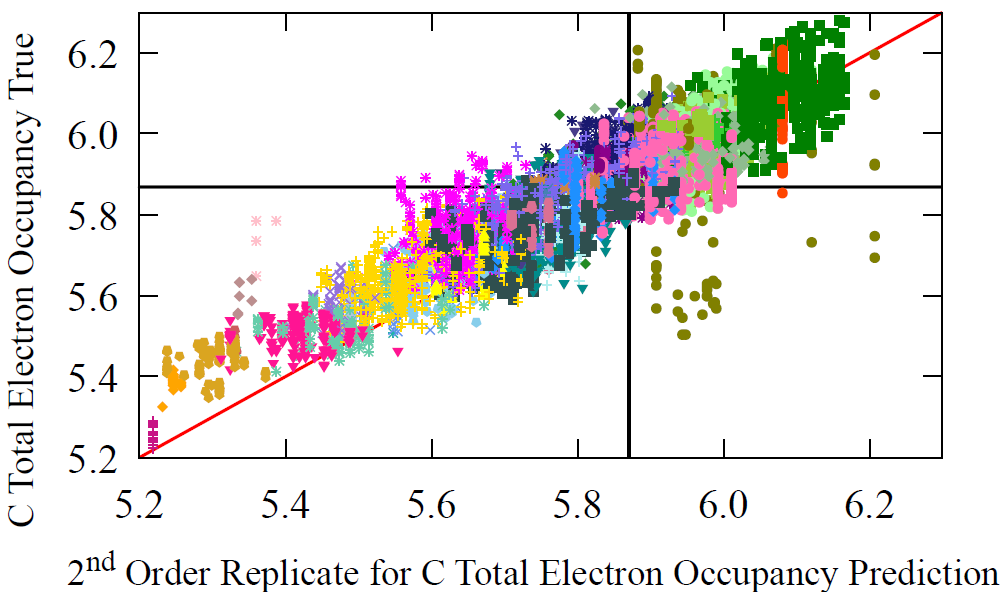

Fig 7 - The prediction performance of reconstructed AFV on carbon’s electron occupancy, over successive refinements (M) of the reconstruction procedure. The zeroth update, i.e. initial guess of our procedure, is the average carbon vector, which fittingly gives the average carbon occupancy prediction shown by the black line. Then the first, second, and third updates are shown in separate figures along with the performance of the original AFV (full GNN pass) on carbon’s total electron density. We can see that over the successive refinements (as M increases), we start to resemble the same profile on carbon total electron density for the original atom vectors (bottom right).
Rather than summarizing the reconstruction performance across all atom vectors, we instead illustrate how a single atom vector prediction evolves through our procedure. As an example, we show the reconstruction of the pKa contribution for the central carbon in trifluoroacetic acid using a depth of one. This molecule provides a clean demonstration of how the updates progressively recover the correct AFV and, in turn, the downstream property.

Fig 8 - Reconstruction of the AFV for oxygen and subsequent prediction of pKa. With each refinement, a deeper neighborhood is integrated into the atom vector reconstruct and the pKa starts to accurately give the trifluoroacetic acid’s pKa.
Using a neighborhood depth of 1, we can track how the reconstructed pKa prediction evolves across refinements. At the first update (M = 1), the model only sees the direct neighbors of the central carbon, so the prediction remains close to the average pKa of an alcohol. By the second update, the neighboring carbon connected to the oxygen begins to recognize that it belongs to a carboxylic acid group, shifting the reconstructed AFV toward the pKa expected for a carboxylic acid. It is only after the third refinement that the influence of the trifluoromethyl group is incorporated. This highly electron-withdrawing substituent stabilizes the conjugate base and dramatically increases acidity, bringing the predicted pKa down to roughly 0.85, close to the true value for trifluoroacetic acid.
We see similar behavior when reconstructing other AFVs. For example, below we show the evolution of hydrogen and carbon NMR predictions for 6H-cyclopenta[b]furan. Here we do not display the subgroup averages at each refinement but instead focus on how rapidly the reconstructed prediction converges to the true value. As expected from the earlier NMR performance results, convergence is achieved by the third refinement (M = 3), reflecting the local nature of the structural information encoded in these AFVs.


Fig 9 - Reconstruction of the AFV for carbon and hydrogen and subsequent prediction of carbon and hydrogen NMR. With each refinement, a deeper neighborhood is integrated into the atom vector reconstruct and the NMR starts to accurately give the true NMR for the atom.
Conclusions
We have demonstrated that the rich, high-dimensional representation produced by a graph neural network (GNN) — the atom feature vector (AFV) space — is not an inscrutable black box but can be deciphered and reconstructed in full. By introducing a simplified, self-consistent message-passing proxy model, we systematically recover the AFV space across molecular graphs. Starting from a crude initial guess, iterative updates align atomic feature vectors with their chemical environments, gradually reconstructing the latent space learned by the original GNN.
This reconstruction also reveals why the AFV space is such a powerful and transferable representation. Because it emerges solely from how local chemical information propagates through message passing, the same vectors can support accurate predictions for many distinct properties, not just the one used to train the original GNN. By recovering this structure through a simplified update scheme, we make clear that the essential engine of GNN chemistry lies in these iterative local refinements rather than in architectural complexity. This provides a transparent foundation for understanding how GNNs learn chemical space and why their learned representations generalize so effectively.