If you’ve ever tried mastering a musical instrument, you’ll realize that, along the way, you naturally absorb the core elements of music theory—chords, scales, and rhythm. Once these fundamentals become second nature, they form a foundation you can seamlessly transfer to other instruments. When you sit at the piano, for example, those same principles guide you, making the transition to a new instrument more intuitive.

Transfer learning in graph neural networks (GNNs) in chemistry operates similarly. As the network grasps the essential building blocks of chemistry in one task, it can apply this deep understanding to tackle entirely new challenges. This enables the model to approach chemistry from a broader perspective, continuously honing its mastery of the underlying principles.

One Model to Rule Them All: Transfer Learning From Graph Neural Networks

Fig 3 - Diagram of transfer learning from GNNs via activation patching. First, we pre-tune a GNN on molecular energies. Second, we pull out the atom activations of a GNN as it tests on molecules. Finally, we use a simpler transfer learning model to predict new properties from the activations.  Our model was a 2-layer feedforward neural network. We also used linear regression, see our publication for full results and details [1].

What is Transfer Learning?

Fig 1 - Learning the fundamentals of music theory

Transfer learning generally unfolds in two key phases. In Phase I, we pretrain a probabilistic model. This pretraining equips the model with a solid foundation of general knowledge—similar to learning the basic chords, scales, and rhythms in music that form the foundation for playing more complex pieces. Once this base is established, the model is ready to tackle more specific tasks.

In Phase II, the model undergoes fine-tuning, which is the core of transfer learning. Here, the pretrained model is adapted to a new task, refining its skills to handle specific data and applications. This can be done in numerous ways, one straightforward way is by retraining the same model but now on a new set of skills.

However, rather than following the traditional path of transfer learning, where the same model is simply pretrained, our Phase II uses a more intriguing approach called activation patching transfer learning. This method bypasses the need for retraining the entire model by instead focusing on extracting and reusing key hidden features from the pretrained model, allowing for more efficient and explainable learning.

Transfer Learning to Atomistic Properties

We’ve already compared assessing a molecule to a doctor evaluating a patient’s health, with molecular energy reflecting the molecule’s stability—its overall health. Let’s extend this analogy: just like the human body has parts with different functions, a molecule has regions with unique roles. One part might be acidic, another magnetic, but they’re all connected by electron density, much like blood flowing through the body. Electron density controls how a molecule donates protons (pKa), responds to magnetic fields (NMR), and even determines the overall energy. These can be referred to as atomistic properties as they can be tied to an atom or a region around an atom, for example, some atoms respond to magnetic fields (carbon), others do not (oxygen), so this is called an atomistic property. 

Just like a doctor might specialize in different parts of the body, transfer learning allows a model to specialize in predicting various molecular properties after initially being trained on one, such as energy. For atomistic properties, this is akin to having a doctor focus on a single part—like a specialist for carbons or oxygens.

In this case, we use a feedforward neural network to make predictions. The input to this model is the Atom Feature Vector (AFV) for each atom, which is obtained from a pre-trained Graph Neural Network (GNN), specifically SchNet. The hyperparameters of this feedforward model, such as the number of layers and learning rate, are tuned to optimize its performance.

The key point is that the AFVs—extracted from the pretrained GNN—act as the starting point for predicting these atom-level properties. The feedforward network then processes these vectors to output a specific property, such as electronegativity or atomic charge.

Fig 4 - The transfer learning model used after training a GNN model. We use activation patching transfer learning, where activations associated with an atom (AFV) are extracted from a previous GNN model and used to learn a new property using a feedforward neural network

As mentioned before, fine-tuning our transfer learning model with specific data is essential. However, thanks to the atom feature vectors, we don’t need nearly as much data as we would from scratch. These vectors already carry inherent chemical knowledge—much like how knowing the chords and scales of music theory allows a musician to play a wide range of songs without starting from zero each time.

In our case, we focused on a balanced set of atomistic properties: pKa, NMR, and electron occupancy—each representing key chemical "specialties" that govern molecular behavior. By fine-tuning the model with data specific to these properties, we’re simply teaching it to specialize, using the foundation it already has.

pKa and NMR: How They Relate to Electron Occupancy — Datasets Used for Transfer Learning

• pKa: This tells us how easily a heteroatom (anything but hydrogen) gives up a proton (a neighboring friendly hydrogen)—kind of like measuring how likely one part of the molecule is to release something important. The more electrons that are pulled away from a hydrogen-donating site, the stronger the acid, and the lower the pKa. It's like how certain parts of the body are more reactive under stress! For the transfer learning data, we used a dataset of 601 experimental pKa values, carefully selected from the IUPAC pKa database for their similarity to QM9 molecules which was used in the pre-tuning phase.

• NMR chemical shifts: NMR measures how an atom responds to a magnetic field, much like how certain parts of the body react to external stimuli. The more electrons that shield the atom's nucleus, the more the NMR signal shifts. This means both pKa and NMR are influenced by the electron density surrounding the atom—like how blood flow impacts different body parts' responses to various conditions. For the transfer learning data, the QM9NMR dataset, containing 10,000 molecules with computed 1H-NMR and 13C-NMR chemical shifts, was used to train the model for accurate NMR predictions.

• Electron occupancy: This is the heart of it all—the actual distribution of electrons in amongst the atoms, influencing both pKa and NMR. More electrons in certain atoms can change how a whole molecule behaves, much like how different organs in the body work together to perform complex tasks. Electron occupancy data for 4,750 molecules from QM9 was generated using computational methods, helping the model understand how electrons are distributed in atoms. We used the GAMESS-US software to compute the electronic structure of these molecules at the same level of theory as QM9 computed properties.

Now let’s delve into the activation patching transfer learning results which were obtained by using a basic 2-layer feedforward neural network with either ‘tanh’ or ‘ReLU’ activation for transfer learning on the abovementioned datasets, after pre-tuning on molecular energy dataset (QM9), which was explained in a previous post.

Activation Patching Transfer Learning

Rather than retraining the full-fledged SchNet neural network on new properties, as done in traditional transfer learning way, we opted for something more exciting: activation patching transfer learning. This technique extracts hidden features from a pretrained model and applies them in a simpler, more explainable model for prediction. By doing this, we gain a deeper understanding of the transfer learning process while using models that are easier to interpret.

Recall from a previous post, we introduced atom feature vectors (AFV), which represent the hidden nodal features a graph neural network (GNN). We discussed that this represents the GNN’s learned information about individual atoms. We also showed how these vectors naturally cluster around functional groups, forming a decision-making framework that explains the model's reasoning on every atom in the molecule—similar to how chords structure a melody in music. This must mean AFVs can transfer learn their knowledge to predict new chemistry, just like any musician can learn a new instructment!

Atomistic Transfer Learning Results

pKa Prediction Results

To the side is a visual comparison between the predictions of our transfer learning model and the actual values of pKa found in our datasets, a.k.a a performance assessment of our transfer learning model. If the model is to be considered accurate, most datapoints have to lie somewhat neatly on a line. The closer they are to the red line in the figure below the greater the accuracy of our transfer learning model. We also show it quantitatively using a measure of root mean squared error (RMSE) which is a measure of how much deviation our predictions our from their bulls-eye value!

Our results show that pKa error can be reduced to within 1.21 pKa units which is within accuracy of most advanced electronic structure methods and compares to employing full-fledged graph neural network training on pKa with thousands of datasets, as was done by Mayr et al. In other words, we have managed to reduce the amount of data and the complexity of the model significantly, without sacrificing much on accuracy.

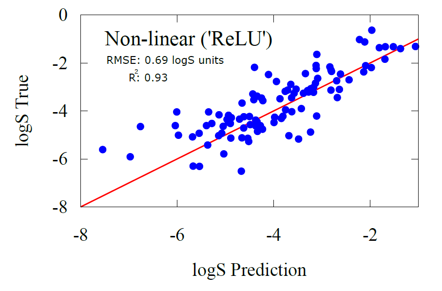
Fig 9 - a) transfer learning predictions vs ground truth for solubility model. b) carbon’s atomwise solubility contributions labelled according to functional groups, labels can be found in Figs 6, 7

We can also start to reveal some interesting trends from our predictions. For example, as expected, the acidity profile is as expected, carboxylic acids have a low pKa due to their readiness to give up a proton easily, whereas groups like alcohols lie on the opposite end of this spectrum. Additionally, alcohols that have nitrogen, like hydroxylamine are more acidic than just plain old alcohols (with carbons) as the nitrogen’s extra electron make the proton more unstable and want to leave. Similarly with alcohols near a double bond are more acidic than plain old alcohols because of the double bond electron donating nature which destabilizes the hydrogen.

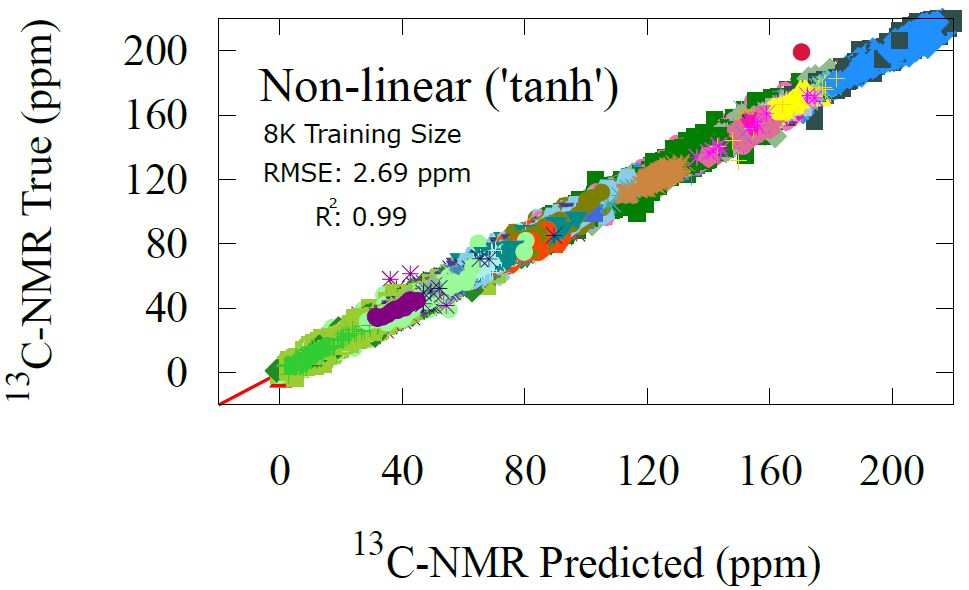
Fig 6 - Performance assessment of the activation patching transfer learning model on carbon NMR predictions, labelled according to functional groups.

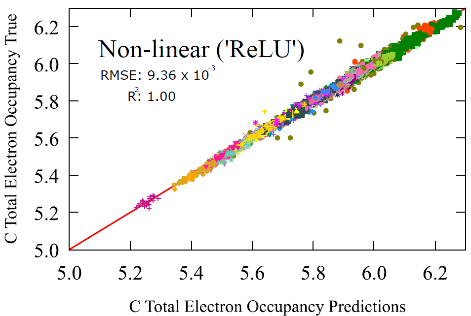
Electron Occupancy Results

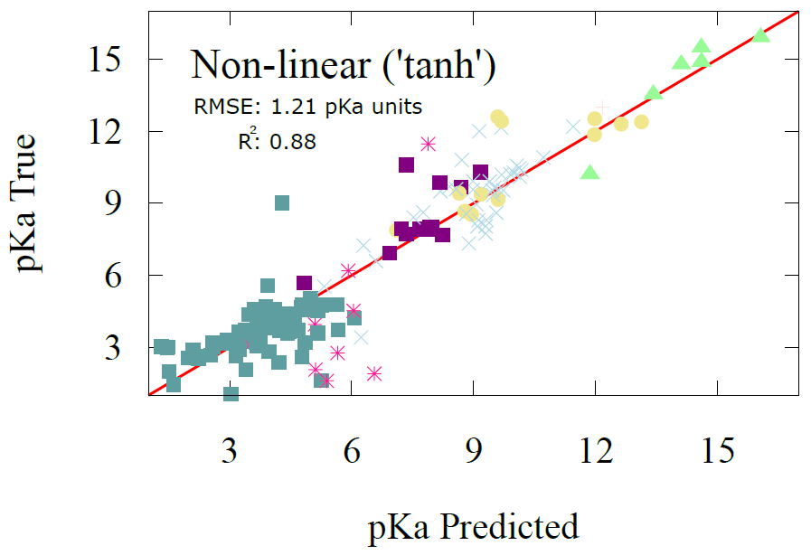
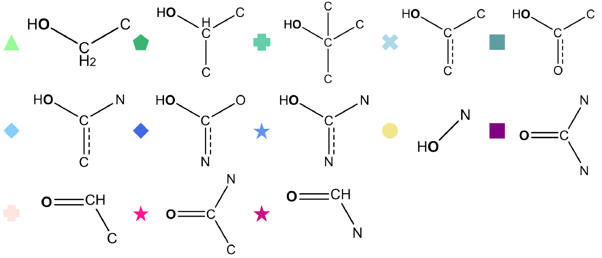
Fig 5 - Performance assessment of activation patching transfer learning model using a basic 2-layer neural network ('‘ReLU’ activation), with functional group labels

NMR Prediction Results

Similarly, we can look at how our transfer model performs on the carbon NMR shifts. Here, we have the advantage of having much data and instantly we find that the transfer learning model shows near perfect alignment and giving a RMSE of just 2.69 ppm which is highly accurate to any other method, including advanced electronic structure methods or full-fledged graph probabilistic models. See out full article below for benchmarking comparisons [1].

Once again, we label the predictions with functional groups to show how the model picks up on the general relationship between functional groups and carbon chemical shifts. That is, this is the core knowledge being used in transfer learning tasks is the original functional group clusters that were learned in the GNN pre-tuning step. This is why the atom feature vectors are so powerful at getting predictions correctly even with very simple models, as they have already picked up on the important chemical concepts to transfer learn.

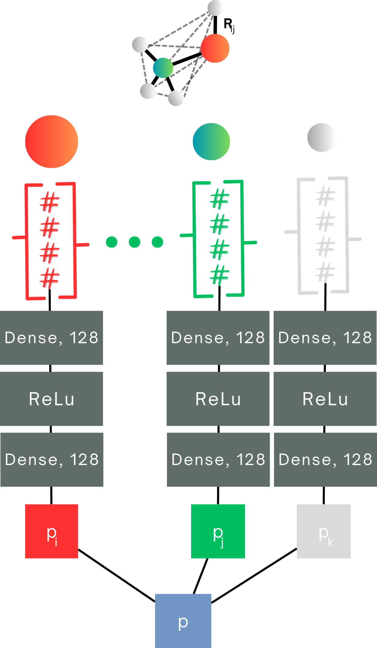
Fig 8 - Transfer learning from AFVs to molecular properties.

Once again, fine-tuning our transfer learning model with specific data is essential, but in this case, we need far less data than we would if we were training an entirely new model. Here, we demonstrate how transfer learning can be fine-tuned for predicting a molecular property like solubility.

Solubility refers to how much of a substance can dissolve in a given amount of liquid, typically water. Think of it like making tea: when you add sugar, it dissolves into the water, becoming part of the liquid. But if you keep adding sugar, eventually, the water reaches a point where no more can dissolve—this is its "saturation point." Solubility measures that threshold.

Different compounds have different solubility limits. For example, salt dissolves very easily in water, making it highly soluble, whereas something like sand does not dissolve at all—it just sinks to the bottom. In chemical terms, solubility is measured either in grams or moles (a unit of amount) per liter of water. Highly soluble compounds, like salt or sugar, can dissolve a lot in water, while less soluble substances, like chalk or oil, don’t dissolve much, if at all.

In our model, solubility is the molecular property we’re trying to transfer learn after pre-training the GNN on molecular energies. Once again, fine-tuning requires data, but much like the musician who has learned music theory this will not be much data. For fine-tuning, we used 800 molecules from the NP-MRD dataset, which contains solubility data for a variety of organic compounds and drugs. We reserved 200 additional molecules for testing, allowing us to assess how well the model performs on new, unseen data. Below are the results of the transfer learning model on predicting solubility for the testing dataset.

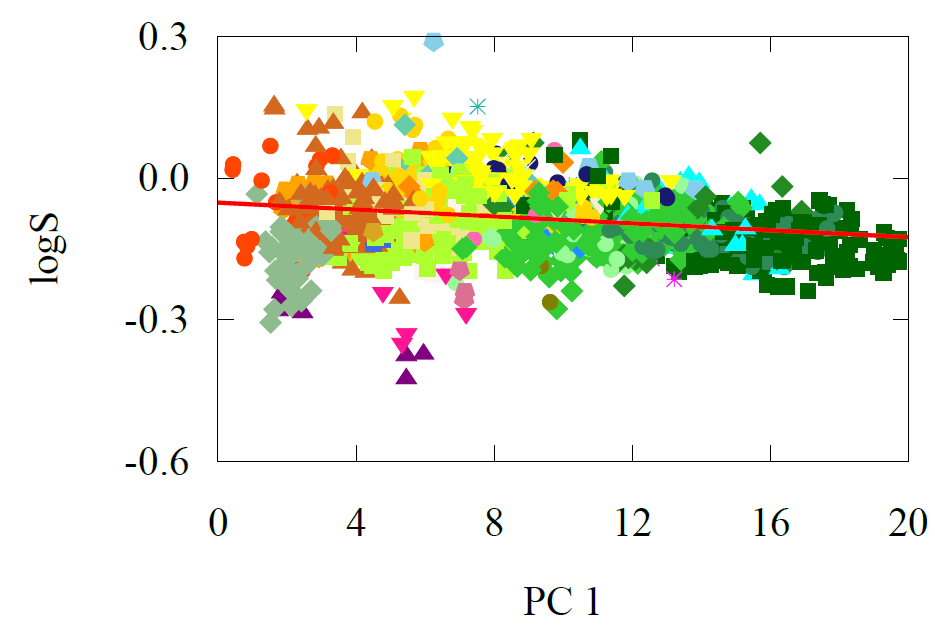
One of the unique advantages of our transfer learning model is that it doesn’t just predict solubility—it allows us to dive deeper and analyze how each atom in a molecule contributes to the overall solubility. By examining carbon atoms, for instance, and grouping them according to their functional groups, we can uncover patterns that reveal how different environments influence solubility.

For example, when we label carbon atoms based on the functional groups they’re attached to, we find a clear profile that organizes these groups according to their solubility. This means the model isn't just making a blanket prediction; it’s learning to interpret specific chemical environments and making decisions on a per-atom basis.

Take carbons with fewer heteroatoms (like nitrogen, oxygen, or fluorine) around them—they tend to make the molecule less soluble, which aligns with our understanding of chemistry. Conversely, carbons with more heteroatoms tend to increase solubility. The model has also picked up on trends regarding symmetry: molecules with highly symmetric structures tend to have lower polarity, and thus lower solubility.

Conclusions

Just as a surgeon learns to specialize in various areas of the body, our transfer learning model has shown it can effectively specialize in predicting diverse chemical properties, such as pKa, NMR, and solubility. This process, which we’ve described as "activation patching," allows us to splice out the critical knowledge learned by Graph Neural Network (GNN) algorithms and apply it to new chemical outcomes—much like a surgeon splicing out the part of your brain that thinks about chemistry and fine-tuning it to learn new tasks.

The success of our model lies in its ability to retain and transfer essential information from its initial training on molecular energies, enabling it to fine-tune efficiently with much less data. We designed two types of transfer learning: atomistic and molecular. In the atomistic approach, the model focuses on predicting properties at the atomic level—think of it like a doctor specializing in a specific organ. Meanwhile, the molecular approach goes a step further, requiring the model to predict overall molecular properties by summing up the contributions of individual atoms.

By leveraging these approaches, our model makes accurate predictions about a wide range of chemical properties with impressive precision. This demonstrates the power of transfer learning in chemistry, extending the capabilities of GNNs beyond their initial tasks and applying them to new, more specific problems. Not only does this provide greater accuracy, but it also allows us to use simpler algorithms and far less data. In a world where training large-scale machine learning models is resource-intensive, this is a huge bonus, especially given the growing awareness that AI's environmental impact could be a significant contributor to climate change in the coming century.

References

For those interested in diving deeper into the details, all connecting citations and results discussed in this post can be found in our full article: [1] A. M. El-Samman, S. De Castro, B. Morton and S. De Baerdemacker. Transfer learning graph representations of molecules for pKa, 13C-NMR, and solubility. Canadian Journal of Chemistry, 2023, 102, 4. This reference provides a comprehensive exploration of how GNNs learn chemistry based on the functional group concept, explains much of the methodology and analysis in this post in much greater detail. Here are some of the other relevant references to this post:

Transfer Learning to Molecular Properties

Building a model that uses activation patching to transfer learn atomistic properties is fairly straightforward. All it takes is isolating the activations in the neural network that correspond to individual atoms—these are the AFVs we have been working with!

Now, when it comes to transferring that learning to molecular properties, things get a little trickier, but it’s still quite manageable! Instead of focusing only on individual atoms, we now need to consider how all the atoms in a molecule contribute to its overall property. Think of it like assembling a team: each atom has a role, and the final outcome (the molecular property) is the result of everyone’s contributions.

In practice, this means we’re still working with a model trained on atom feature vectors. However, instead of stopping at the atom-level, we’re adding up the impact of each atom to get a total molecular property. The model doesn’t just look at individual players—it’s now playing a full team sport!