

How Graph Neural Networks Learn Molecular Representations from Quantum Mechanics
Graph neural networks compress the enormity of quantum chemistry into compact description of molecules. The distance between these learned molecular descriptors define a fine measure of molecular similarity, while enabling precise downstream learning — article link
Physics gives us the fundamental laws governing how atoms interact, and in principle these laws can predict molecular behavior exactly via first-principles calculations. But even for small molecules this is a staggering computational challenge: solving quantum mechanics scales poorly, quickly becomes infeasible, and demands enormous memory and computation.
Graph Neural Networks GNNs [2 - 6] sidestep this obstacle by training on systems that have already been solved through exact or approximate methods. Crucially, GNNs encode molecules using a similar inductive bias of chemical computations (decoupling electronic and nuclear components of a molecule). Nuclei can be represented as nodes (particles) with the edges being the natural distance between the nodes.
The training process enables a GNN to encode each node in a graph into a vector representation that reflects not only the atom’s identity, but also the effect of neighboring nodes and their distance. In effect, from training on quantum-mechanical data, the model constructs an internal coordinate system that compresses the many body solutions into a function of local environments.

Non-linear projection techniques are capable of revealing complex, high-dimensional structures that linear methods like PCA might miss, but they come with important caveats: non-linear projections often distort distances and relationships in ways that are difficult to predict, so care must be taken when interpreting the results.
One widely used method is t-distributed Stochastic Neighbor Embedding (t-SNE) [9] shown to the side for the oxygen AFVs of 10,000 QM9 molecules. t-SNE preserves local neighborhoods—points that are close in the 128-D space remain close in the 2-D projection—making it excellent for visualizing fine-scale structure. However, long-range distances are unreliable, and the global arrangement of clusters can sometimes appear arbitrary or even misleading.
Despite these limitations, t-SNE is extremely effective for revealing local organization in the AFV space, as seen in the sharp clustering of functional groups and the broader chemical families they form.
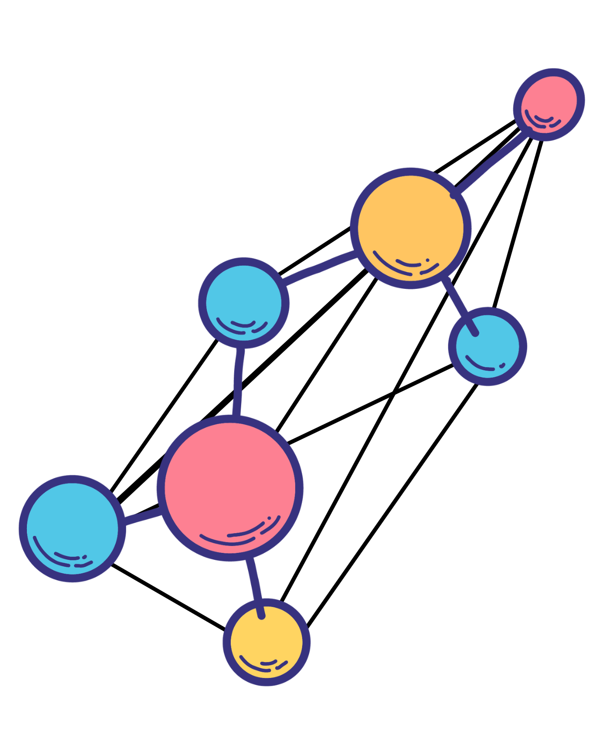
Fig 1 - A graph is formally defined as a mathematical object composed of 1) nodes and 2) pairwise edges.
These learned atomistic representations, often called learned descriptors, can be used to predict molecular properties and behaviors and to propose new molecular structures at a fraction of the computational cost of first principles electronic structure methods.
In this work, we examine what these learned descriptors encode, how chemical information is organized in the latent space, and why this organization is scientifically meaningful. Our goal is to interpret the latent space of graph neural networks through a rigorous and explainable framework, transforming them from opaque function approximators into models grounded in recognizable chemical and physical principles.
A key result is a direct connection between learned GNN descriptors and molecular similarity measures long used in cheminformatics. Unlike traditional approaches that rely on hand crafted descriptors, graph neural networks learn these representations directly from data, with evidence that they capture molecular similarity more faithfully than pre designed alternatives.
At the very first layer, the trained graph neural network encodes almost nothing about molecular structure. Each atom is identified only by its element type. Concretely, the atomic number Zi is mapped through a predefined or a learned initial atom feature vector (AFV).
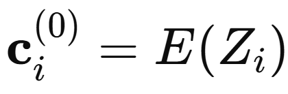
At this stage, the AFV descriptor simply separates carbons from oxygens, nitrogens, fluorines, and so on. It is a learned periodic table: a set of vectors that lets the model distinguish elements but not yet their structural environment.
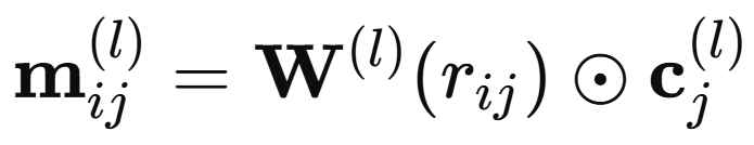
All information about bonding and geometry enters through the subsequent interaction layers. In a general interaction layer l, atom i receives messages from its neighbours j that depend on both the current neighbour representation and the interatomic distance. The distances are first expanded in a set of radial basis functions:
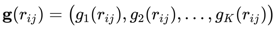
This expands each interatomic distance into a richer set of basis features that a neural network can more effectively process (e.g., rather than just processing single number, the distance, to pass through). The resulting feature vector is then passed through a small neural network that generates a distance dependent filter.
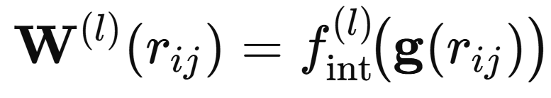
This filter then modulates the neighbor nodes’ representation through elementwise multiplication. Practically, the radial basis expansion is compressed by several dense layers until it matches the dimensionality of the nodal representation space, the AFV.
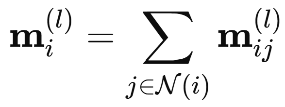
and the messages from all neighbours are summed to pool all contributions
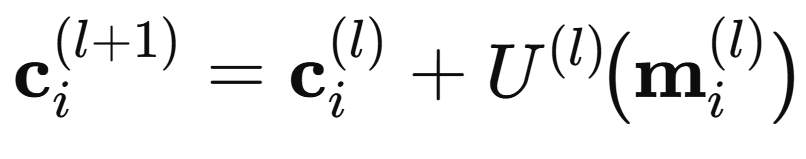
Finally, atom i updates its own representation through a learned update network
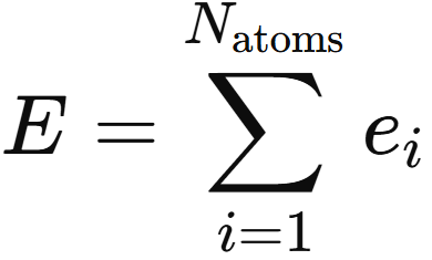
The interaction module is repeated a user-chosen number of times. Once the interaction layer produces the updated AFVs, the model needs a mechanism to process these vector representations into the target property, a scaler. The output network performs this role. Applied identically to each AFV, it infers atomic contributions that sum to the global observable, and through backpropagation it continually shapes how the AFVs are built themselves
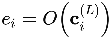
At last, the model ties the entire representation learning process to the target physics through the final summation of all atomwise contributions produced by the output network.
At the start of training, the AFVs, and the messages that update them are essentially random and do not encode a precise fitting of the output property. After optimization on a physically meaningful target—such as exact or approximate electronic energy solutions of first-principles approximation—the interaction and update networks learn how to adjust messages, AFVs, and how to use them in a way that results in precision to the final property.
We trained such a GNN on the QM9 dataset—~134k DFT-computed internal energy values at 0 K—and obtained a highly accurate model, reaching a cross-validation error of only 0.02 meV. [1] Yet despite this remarkable precision, the GNN’s latent space—encoded in the atom feature vectors (AFVs)—remains largely opaque. Given all this processing and layers and message-passing ineteractions, it is not entirely clear what description is being built by the GNN, what does the final atomistic representation look like? how does it work to make precise downstream predictions?
We will dive in to see this by using several dimension reduction techniques on the learned AFV description of a set of organic molecules. These techniques will reveal the connection between GNN learned descriptors and molecular similarity measures of cheminformatics while also revealing interesting trends of c
What the Learned Representations Actually Are: Atom Feature Vectors and Their Organization
A central challenge with GNNs is that the latent model used to predict molecular energies is often difficult to interpret. It is not clear whether the message-passing steps that construct the atom feature vectors (AFVs) produce a chemically meaningful latent space, or whether they simply form a non-interpretable description, that just happens to yield strong predictive performance.
The other problem is that the atom feature vectors themselves contain a large number of parameters—each AFV in our trained model is a 128-dimensional vector. Even if the message-passing process organizes these vectors in a meaningful way, such a high-dimensional space is essentially impossible to interpret directly. Thankfully, there are techniques that allow us to project these high-dimensional embeddings into lower-dimensional spaces while preserving their structural relationships. These methods—such as PCA, t-SNE, and other dimensionality-reduction tools—enable us to visualize and analyze the organization of the AFVs and assess whether they encode chemically meaningful patterns.
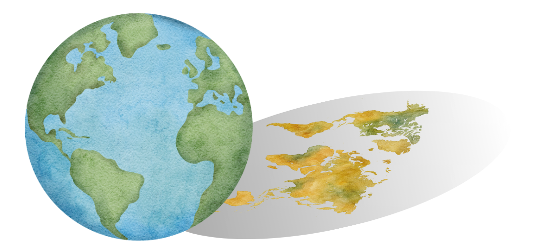
Fig 2 - projecting earth 3D surface onto a 2D map inevitable introduces distortions.
Each of these techniques comes with its own strengths and weaknesses. The fundamental challenge is the trade-off between information preservation and information loss. Any reduced-dimensional representation is, at best, a shadow of the original 128-dimensional space—an approximation that inevitably discards some detail. However, these “shadows” are still extremely useful: they can preserve important aspects of the organization of the data, such as distances between points, topology, and overall distribution. By projecting the AFVs into these lower-dimensional spaces, we gain a way to visually interpret how the representations are organized and assess whether they reflect meaningful chemical structure.
Linear vs Non-Linear Low Dimensional Projections of the Embedding Space
The first technique we consider is Principal Component Analysis (PCA). [8] PCA is a linear dimensionality-reduction method that identifies the directions of greatest variance in the 128-dimensional AFV space and projects the data onto those axes. In other words, it finds the two-dimensional plane that captures the most variation in the high-dimensional data, providing the most informative linear “view” of the space. Think of it like photographing a 3-D house from the angle that shows the most of its structure—the view that best preserves the shape and features of the house in a 2-D image, e.g., landscape front view.
Because it is linear, PCA preserves global structure and provides a straightforward, interpretable mapping. However, its linearity is also its main limitation: PCA cannot “unfold” or separate complex non-linear relationships embedded in the high-dimensional space. If chemically meaningful clusters are arranged in a curved, intertwined, or otherwise non-linear fashion, PCA will fail to tease them apart—the 2-D linear projection is limited by its simplicity.
How Graph Neural Networks Model Chemistry
Fig 2 - A simplified GNN diagram focused on the message passing operations between atom feature vectors AFVs, which represent the nodal elements of the molecular graph.

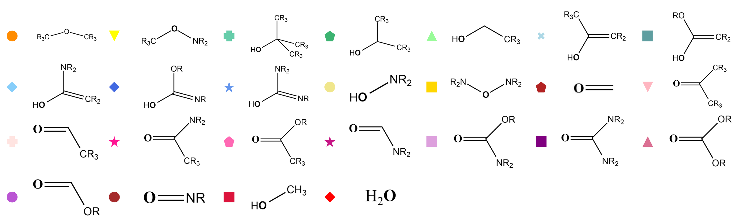
Fig 5 - t-SNE’s 2-D projection of the 128-D oxygen atom feature vectors (AFVs) of the SchNet[2-5] graph neural network, while being tested on QM9 dataset.
Confirming High-Dimensional Separation with Linear Discriminant Analysis (LDA)
To verify whether the functional-group clusters suggested by t-SNE truly exist in the original 128-D AFV space, we use Linear Discriminant Analysis (LDA). [10] LDA is a supervised method that finds linear combinations of the input features—here, the 128-D AFVs—that maximize separation between predefined classes while minimizing variation within each class. Unlike PCA, which is unsupervised and focuses solely on overall variance, LDA explicitly leverages class labels to identify directions where groups are most distinguishable.
It is important to note that LDA does not preserve all original distances. By projecting the high-dimensional data into a lower-dimensional subspace, some geometric relationships are intentionally distorted. This distortion is purposeful: LDA prioritizes class separability over exact distance preservation, giving a view of data where clusters are as distinct as possible.
To apply this to our data, we labeled each AFV by its corresponding functional group (e.g., alcohols, carbonyls, amines, etc.) and trained LDA on the 128-D AFVs from 10,000 QM9 molecules. The resulting LDA projection reveals striking separation between functional groups, confirming that the clusters observed in t-SNE are not artifacts of the non-linear projection. Even in the linear 128-D space, groups such as alcohols, hydroxyls near carbonyls, and carbonyl-containing species are clearly distinguishable, and their relative positions match the chemical similarities suggested by t-SNE.
Applying LDA to the AFVs, labeled by functional groups defined up to two bonds away, such as primary alcohols, esters, and carbonates, reveals clean separation between classes in the original 128 dimensional space. The near perfect classification confirms that the clusters seen in t SNE reflect genuine high dimensional separability rather than an artifact of nonlinear embedding.
Although LDA stretches and rotates the space to maximize class separation, it is still a linear transformation. Like PCA, its axes are only coordinate mixtures of the original AFV features. Because of this linearity, LDA cannot invent well defined boundaries if the original 128 dimensional representations do not already contain them. The resulting neat separation therefore demonstrates that the model has learned a chemically meaningful organization of functional groups.

Some exceptions do appear: because t-SNE stretches or compresses long-range distances to squeeze the 128-D geometry into 2-D, certain groups that are moderately similar in the original space may end up unexpectedly far apart or wrapped around other clusters. For example, α-hydroxyl groups—which sit between alcohols and carbonyls in both the 128-D distance distributions and in the linear PCA projection—are placed closer to carbonyls than to alcohols in the t-SNE map. Nevertheless, t-SNE still captures much of the global chemistry: N–O–N groups lie near C–O–C groups, and H–O–N clusters sit close to H–O–C clusters, reflecting meaningful chemical similarity
The striking aspect of the t-SNE projection is the presence of clear “empty space’’ separating functional-group clusters. This raises an important question: does this separation truly exist in the original 128-D AFV space, or is it an artifact of the non-linear projection? Neither the PCA view nor the raw 128-D distance distributions make this immediately obvious. To answer this quantitatively, the next section applies a linear classifier—Linear Discriminant Analysis (LDA)—to the functional-group–labeled AFVs, confirming that the high-dimensional space is genuinely as well-separated as t-SNE suggests and not as the PCA suggests.
Fig 6 -Top Left: 2-D PCA projection of the 128-D AFV space for 10,000 QM9 molecules, showing clear clustering by chemical group and a meaningful global arrangement of those groups. Top Right: Because PCA distorts true distances, we plot the actual 128-D Euclidean distances from the oxygen in propargyl alcohol to all other oxygen-containing molecules confirming global organization (e.g., alcohol —> alcohol-carbonyl —> carbonyl). Bottom Right: A zoom-in highlights a smooth, fine-grained relationship between structure and 128-D distance for molecules closely related to propargyl alcohol. Bottom Left: A PCA zoom-in on straight-chain alcohols shows that the distance–structure trend is still visible in 2-D, but slightly distorted. In the true 128-D space, distances decrease smoothly with increasing chain length, whereas PCA “squishes” nonlinear geometry into a linear plane, bending these relationships slightly, motivating the need to use non-linear projections.
Above is the PCA projection of the 128-dimensional AFV representations for 10,000 molecules in our test set. While the clusters are not immediately obvious without labeling the AFVs by their associated chemical groups, the projection still reveals a notable degree of organization. This suggests that the high-dimensional 128-D space itself is structured in a meaningful way.
The AFVs not only cluster according to chemical groups, but the functional groups themselves are organized in a way that reflects their relative similarity, showing global structure in the AFV space. For example, alcohol groups cluster together and near other hydroxyl-containing groups, while hydroxyl groups adjacent to carbonyls are positioned close to carbonyl-type groups—amides, esters, carbonates—forming a neatly organized map, much like a library with related sections placed near each other.
Zooming in on linear-chain alcohols—methanol, ethanol, propanol, butanol—we see that their AFVs draw progressively closer in the PCA projection. But this 2-D view masks a key fact: in the true 128-D space, the distances between successive alcohols decrease smoothly and monotonically with chain length. PCA, being linear, cannot follow the nonlinear geometry of the AFV manifold, so the 2-D distances become slightly distorted—for example, propanol-to-butanol appears farther apart in 2-D than ethanol-to-propanol, even though the 128-D distances decrease continuously. These distortions underscore the limits of linear projections and motivate using nonlinear methods like t-SNE to better reveal the underlying structure of the AFV space.


Fig 8 - LDA confusion matrix on the atom feature vectors classifying chemical environments.
Conclusions
Interpreting a 128 dimensional representation requires multiple lenses, each sensitive to different geometric truths. The linear methods, PCA and LDA, respect the global structure of the AFV space because they can only rotate, stretch, or compress along mixtures of the original coordinates. PCA reveals the broad scaffolding of chemical similarity by preserving large scale distances, while LDA tests whether functional classes are truly separable without the freedom to invent nonlinear boundaries. Their agreement shows that the high dimensional space already contains clean, chemically meaningful partitions.
Non linear methods like t SNE highlight a different aspect of the geometry. By focusing on preserving local neighborhoods rather than global distances, t SNE exposes the fine texture of the AFV manifold: the subclusters within functional groups and the smooth transitions across related environments. Even though t SNE may distort long range relationships, its sensitivity to local structure reveals details that linear projections necessarily flatten.
When these perspectives are combined, a coherent picture appears. PCA outlines the global map, LDA confirms the true boundaries, and t SNE fills in the local anatomy that makes the representation chemically expressive. Each method shows a different shadow of the same high dimensional object, and their mutual consistency demonstrates that the network has learned a latent space whose organization mirrors the logic of chemistry itself.
References
For those interested in diving deeper into the details, all connecting citations and results discussed in this post can be found in our full article:
[1] A.M. El-Samman, I.A. Husain, M. Huynh, S. De Castro, B. Morton, and S. De Baerdemacker. 3(3):544–557, 2024
[2] K. T. Schütt, P.-J. Kindermans, H. E. Sauceda, S. Chmiela, A. Tkatchenko and K.-R. Müller, arXiv preprint arXiv:1706.08566, 2017.
[3] K. T. Schütt, F. Arbabzadah, S. Chmiela, K. R. Müller andA. Tkatchenko, Nature communications, 2017, 8, 1–8.
[4] K. Schutt, P. Kessel, M. Gastegger, K. Nicoli, A. Tkatchenko and K.-R. Muüller, Journal of chemical theory and computation, 2018, 15, 448–455.
[5] K. T. Schütt, H. E. Sauceda, P.-J. Kindermans, A. Tkatchenko and K.-R. Müller, The Journal of Chemical Physics, 2018, 148, 241722.
[6] R. Zubatyuk, J. S. Smith, J. Leszczynski, and O. Isayev, Science Advances 5, eaav6490 (2019).
[7] R. Ramakrishnan, P. O. Dral, M. Rupp and O. A. Von Lilienfeld, Scientific data, 2014, 1, 1–7.
[8] H. Abdi and L. J. Williams, Wiley interdisciplinary reviews: computational statistics, 2010, 2, 433–459
[9] L. Van der Maaten and G. Hinton, Journal of machine learning research, 2008, 9, year.
[10] A. M. Martinez and A. C. Kak, IEEE Transactions on Pattern Analysis and Machine Intelligence, 2001, 1, 228-233