Transfer Learning From Graph Neural Networks Trained on Quantum Chemistry
Graph neural networks trained on quantum chemical data learn a fine grained, compressed representation of molecular physics. This representation can be reused as a starting point for transfer learning, enabling accurate models on fewer than one thousand data points and addressing the challenge of generalizable learning with small datasets — link to the CJC award winning article
The monumental advantage of quantum chemistry lies in its ability to predict the behavior of complex materials from first principles, without relying on experimental data. In effect, it generates theoretical data directly from physical law. The challenge, however, is the sheer size of these solutions.
Many body methods treat a system as a collection of interdependent particles, where each particle interacts with every other one. This quickly becomes memory intensive because every interaction must be accounted for explicitly. The number of interactions grows rapidly with system size. Even a modest molecule like caffeine, which contains 192 electrons, has (192×191)/2=18,336 distinct symmetric electron electron interactions. Each of these interactions is not a single value, but a function spanning a vast space of possible states. As a result, storing the full many body solution for caffeine quickly becomes computationally infeasible. In short, so while generating data is cheaper than experiment, it is still not ideal scenario as it scales poorly with computational costs.
Machine learning offers a complementary set of strengths and limitations. Rather than solving the full interacting problem, machine learning builds compact representations of a combinatorial space. In this sense, machine learning is memory light, but it is data hungry. The amount of data required depends on the complexity of the problem and the model, but a common rule of thumb is that one needs at least ten times more data points than tunable parameters. For a typical graph neural network with roughly one thousand parameters, this implies a minimum of ten thousand labeled data points, and in practice often far more.
In summary, many body physics is memory hungry but can generate data without prior examples, while machine learning relies on compact representations but requires large amounts of data to learn them.
The real power emerges when these two worlds are combined. When a symmetry-informed machine learning model (e.g., SchNet GNN), or even better a physics-informed one, is trained on quantum chemical solutions, it learns a compact representation that encodes much of the underlying physics in a memory efficient form. This pretrained representation can then be reused as a starting point for new learning tasks, avoiding expensive quantum calculations and dramatically reducing data requirements. In many cases, downstream models can be trained on fewer than one thousand data points while retaining high accuracy. In this way, transfer learning directly alleviates the data hunger of machine learning by embedding physical knowledge into the model from the outset.

Fig 2 - Pianist learning the piano and a model of musical theory to transfer to new instruments.

Fig 4 - transfer learning overview using GNN-built represenation of atoms
pKa Transfer Learning Results
pKa is a measure of acidity in organic acids, the lower the pKa the more acidic a site is which chemically means it gives up a proton very easily to other acceptors. We trained two downstream models for predicting pKa: a linear regression model and a one-layer neural network, both described earlier. Because pKa is a site specific property, the AFV used as input corresponds to the heteroatom capable of donating a proton, typically oxygen or nitrogen. Although one could instead select the proton’s AFV directly, we deliberately used a nearby heavy-atom site to demonstrate that the representation is robust even when sampled slightly away from the exact reactive center.
The linear regression model achieves an RMSE of 1.44 with a correlation coefficient of 0.83. The one-layer nonlinear model improves performance only modestly, yielding an RMSE of 1.21 and a correlation of 0.88. Despite their simplicity and the limited training data available, these results fall within the accuracy range of advanced electronic structure methods and compare favorably to full GNN models. For example, Mayr et al. reported an RMSE of 0.82 after training a GNN on 714,906 datapoints. Here we obtain competitive performance using fewer than 500 training points and a drastically simpler model, illustrating the efficiency and predictive strength of the AFV representation.
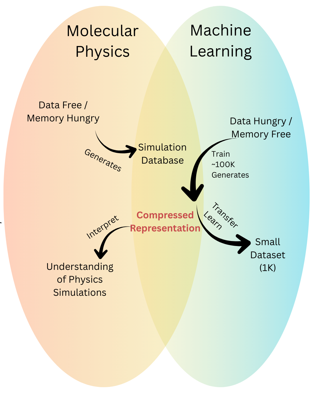
Fig 1 - Physics on the left, data driven models on the right. A ML trained on physics sits in the middle (e.g., GNN), turning memory heavy calculations into a compact representation that small datasets can reuse.
Transfer Learning from Compact Representations
Transfer learning is a broader idea than its use in AI. If you have ever learned a musical instrument, you know it is impossible to progress by memorizing finger movements alone. As you practice, your mind inevitably absorbs elements of music theory chords, scales, rhythm, and harmonic structure. You are not just repeating motions; you are building an internal model of how music works. Modern AI systems behave similarly. When trained on a task grounded in a fundamental domain such as molecular physics, they do more than memorize examples. They begin to construct an internal representation of the underlying principles, which can then be reused for new tasks. This is the essence of transfer learning.
There are two main forms of transfer learning. The first is the familiar one: take a pretrained model and retrain the entire model on a new task. This is like asking a pianist to learn guitar by relearning every piano movement on the guitar. In AI terms, it means fine tuning all of the GNN’s parameters on a new property or dataset. This approach works, but it is inefficient and data hungry because GNNs contain many parameters that must be reoptimized. And musically, it makes no sense either. You do not play guitar by mimicking piano keystrokes. A guitar asks you to strum, bend notes, play riffs, and improvise. Relearning everything from scratch misses the whole point.
The second form of transfer learning is far more efficient. Instead of retraining the entire model, we extract only the learned representation—the internal features the GNN built during training. These features, the atom feature vectors (AFVs), as shown in a previous post, encode meaningful chemical principles. We then use this representation as the input to a new, lightweight model for a different property. This is similar to a musician learning a new instrument not by copying the exact motor patterns used on the piano, but by drawing on their existing understanding of musical theory. The underlying knowledge of harmony, rhythm, and structure transfers, allowing them to learn the guitar with far less time and effort. In the same way, using the AFVs allows new chemical models to be trained with dramatically fewer data and resources.
This representation level reuse dramatically reduces the amount of data needed for a new chemical task. Rather than teaching a model quantum chemistry again, we begin from a space that already encodes it. As we will show, this allows accurate models to be trained with fewer than one thousand data points, providing a practical path forward for small dataset learning in chemistry.
Regardless of which transfer learning method is used, there are two phases to transfer learning. Phase I is the pre-training phase this is the model you spend a lot of resources on, the model you have a lot of data for. In our case, this the quantum chemical simulation data. This phase generally requires lots of data points, for GNN model nearing on ~100 K datapoints. From this model a compact representation is built which can be used in the second phase. in Phase II, the model itself or a new (leaner and more appropriate model) is fine-tuned from the compact representation already built from Phase I.
Transfer Learning on pKa, NMR, Solubility, and Electron Density
We can also uncover several interesting chemical trends from our predictions. At a coarse level, the model recovers familiar acidity patterns: carboxylic acids cluster at low pKa, alcohols appear at much higher values, and substituents such as nitrogen shift alcohols toward greater acidity by destabilizing the bound proton. Similar shifts occur for alcohols adjacent to double bonds, where conjugation and electron donation alter the proton’s stability. Yet the more striking patterns emerge when we move beyond simple functional group labels. The AFV space does not reproduce a rigid textbook classification but instead captures continuous variations within each class. For instance, hydroxylamine shows two distinct pKa regions, likely reflecting whether the group participates in aromatic stabilization. These long range and environment dependent effects arise naturally from the message passing process that constructed the AFV representation during pretraining.
These trends highlight the strength of the AFV space as a chemically aware latent representation. Because it was shaped by quantum mechanical data during pretraining, the AFV space already encodes a nuanced map of chemical environments. Downstream tasks such as pKa prediction can then leverage this structure with minimal data, allowing subtle structural and electronic effects to be recognized even when functional groups alone would fail to discriminate them.
Carbon Electron Occupancy Transfer Learning Results
Electron occupancy, or the number of electrons around an atom, is a fundamental electronic property of molecules, reflecting how electron density is distributed around the molecule. It plays a central role in determining many other chemical observables. For carbon in particular, electron occupancy governs its local reactivity, the stability of intermediates, its susceptibility to electrophilic or nucleophilic attack, and even measurable quantities such as NMR shielding and pKa. Because it encodes how electrons respond to their chemical environment, occupancy acts as a foundational descriptor from which more complex properties emerge. Accurately learning or reconstructing this quantity therefore provides insight not only into electronic structure itself but also into the broader network of chemical behaviors that depend on it.
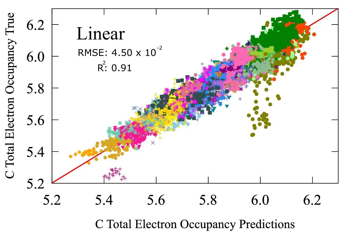
The linear regression model achieves an error 0.0450 with a correlation coefficient of 0.91, already signifying strong qualitative relationship. The non-linear model achieves a scale in magnitude lower in accuracy giving 0.00936 with a correlation coefficient of 1.00. This is a property that is traditionally derived from the electronic structure calculation of a molecule. A mechanistic model rather than a probabilistic model. But here we show that a probabilistic model can obtain almost identical results with the mechanistic ones.
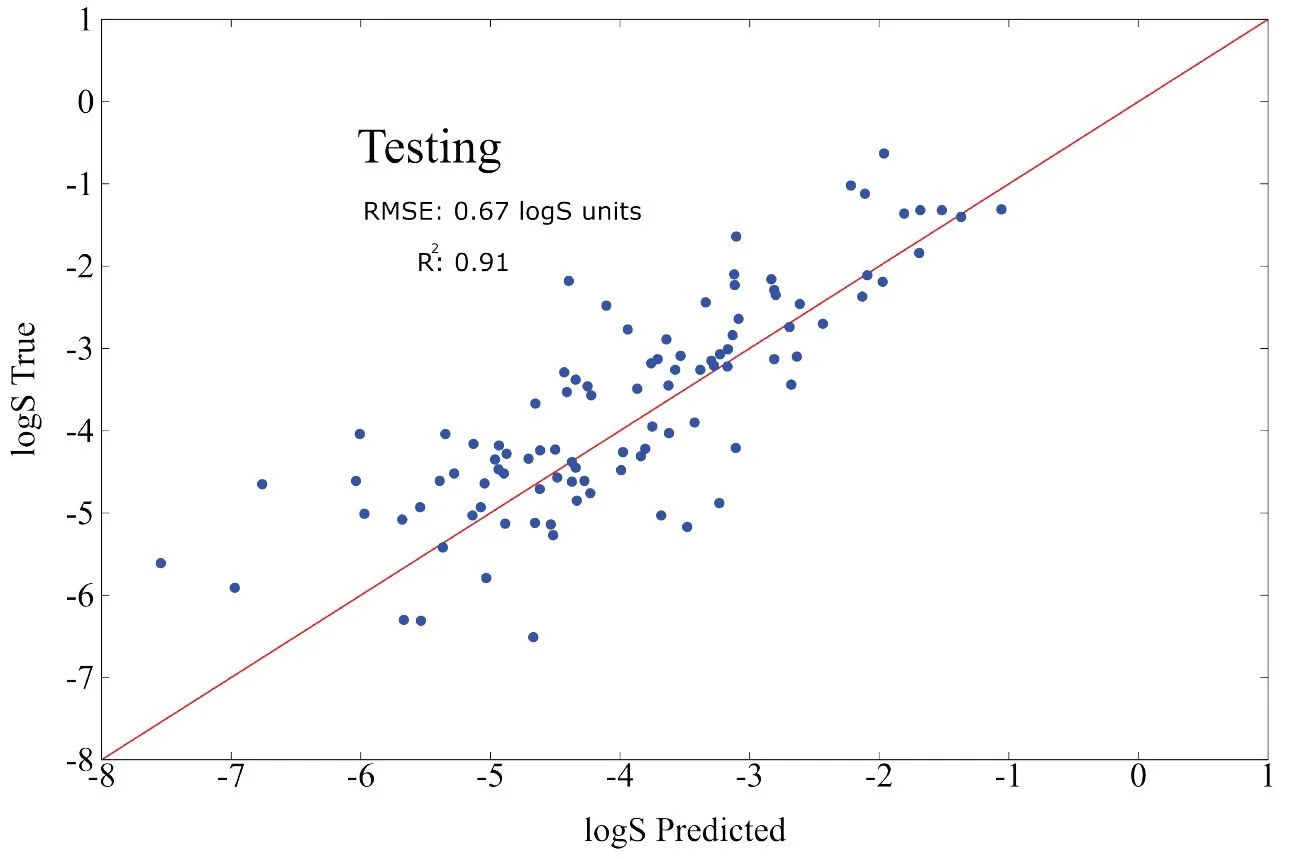
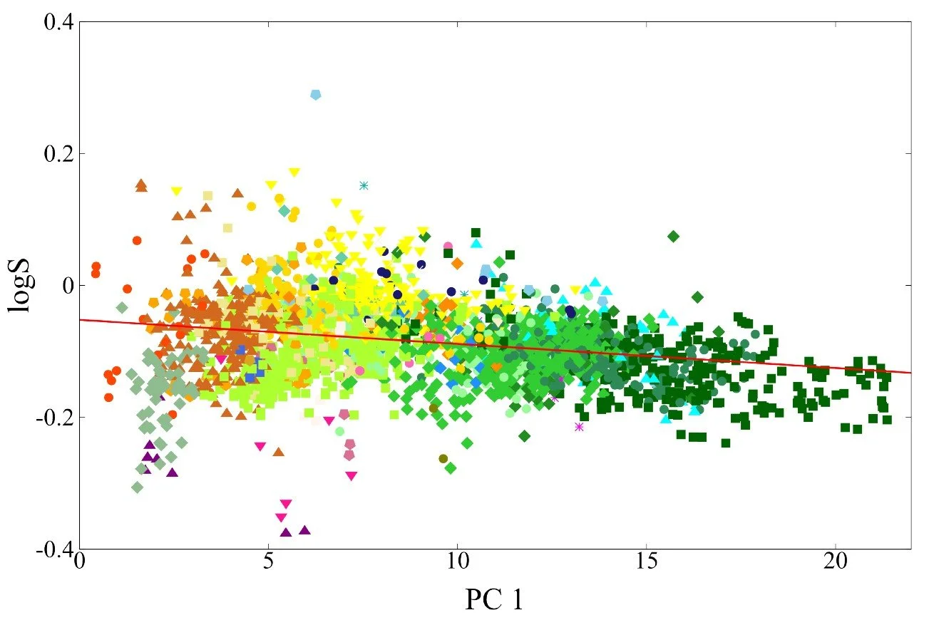
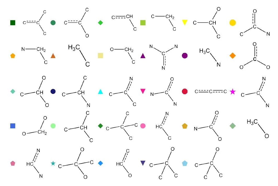
Fig 9 - Transfer learning performance on solubility logS of a test set of 160 molecules from the NP-MRD database. Below it is a figure of carbon contributions to the logS plotted against first principle axis.


Transfer Learning From a Pretrained Representation, Abandoning the Full GNN Pass
Fig 3 - two phases to transfer learning, pre-tuning and fine-tuning
To demonstrate the power of transfer learning in the fundamental domain of quantum chemistry, we adopted a two-phase approach. In Phase I (pretraining), we trained a message-passing GNN on the 134 thousand molecules of the QM9 dataset. This phase teaches the model a generalizable chemical representation. For details on both the dataset and the GNN architecture, see the previous post.
In Phase II, we extracted the pretrained representation—the atom feature vectors (AFVs)—which were analyzed extensively earlier. Instead of performing a full GNN pass for each new property, we reuse these AFVs as fixed inputs for downstream learning tasks. This allows us to learn new chemical properties such as pKa, NMR shifts, and solubility using fewer than one thousand datapoints, highlighting the efficiency and data economy of the AFV representation.
The downstream models used in Phase II were intentionally simple: either linear regression or a single-layer dense neural network. For local properties, the input is the AFV corresponding to the atom, which is sufficient to capture local chemical trends. For size-extensive properties such as solubility or total electron density, the model processes AFVs for all atoms and pools their contributions to match the molecular target. This setup shows that once AFVs are learned during pretraining, even very simple models can leverage them to predict a wide range of chemical properties with high accuracy.
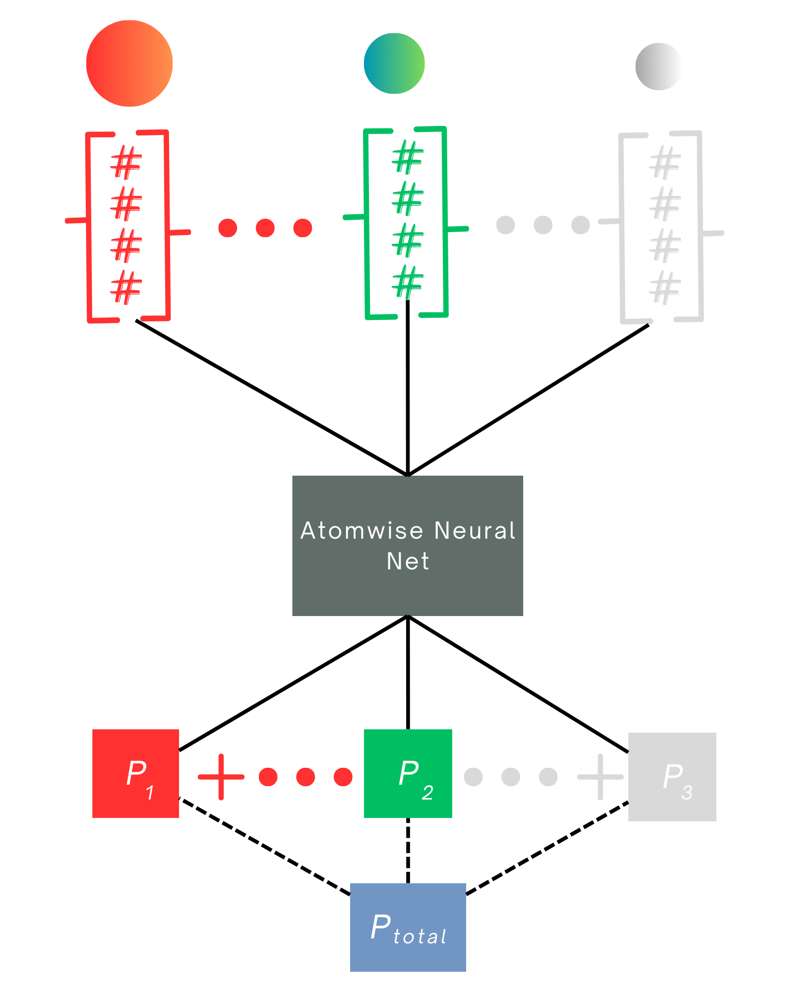
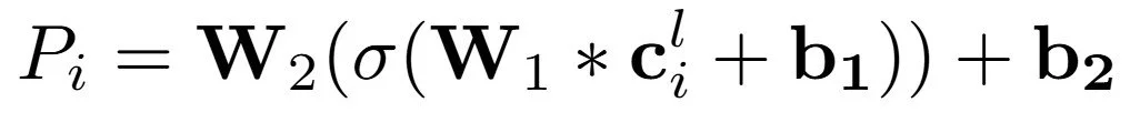
We define three main downstream models that operate on the AFV representation. The first is a simple linear regression from AFV to property. The second is a one layer dense neural network, which we refer to as the atomwise neural network. It consists of a linear layer, a non linear activation such as tanh, and a final linear layer to map the output to the property value.
The third model is used for size extensive molecular properties such as solubility or total electron density. In this case, the atomwise neural network is applied to every atom’s AFV to generate atomwise contributions that are then pooled by summation to produce the total molecular value. The model is trained on the molecular target, ensuring that the learned atomwise contributions scale appropriately with molecular size and composition.
We trained downstream models for four chemically distinct properties: pKa (acid reactivity measure), NMR shifts (an electromagnetic property), solubility (a thermodynamic property), and total electron density (an electronic property). Local properties such as pKa and NMR shifts were learned using either model architecture 1 or 2, while the molecular properties electron density and solubility were learned using model architecture 3.
Each downstream dataset was intentionally kept small to highlight a central point. These models are far less data hungry than full GNNs and are therefore well suited to experimental chemistry settings, where high quality data are often limited. The training and testing splits are as follows:
pKa: 400 training and 100 testing points from the experimental IUPAC pKa database
NMR Dataset 1: 481 training and 120 testing points from NMRShiftDB2
NMR Dataset 2: 8000 training and 2000 testing points from QM9NMR
Solubility: 640 training and 160 testing points from the NP MRD database
Electron density: 3800 training and 950 testing points from DFT calculations (B3LYP/6-31G(d,p))
With the exception of the second NMR dataset and the electron density dataset, all training sets contain fewer than one thousand datapoints, a regime where standard deep learning models typically overfit. We include the larger NMR set to illustrate how dataset size affects the performance of linear and non linear downstream models. A notable outcome is that linear models rapidly underfit as the dataset grows, demonstrating that even simple non linearity offers significant additional flexibility when more data are available.
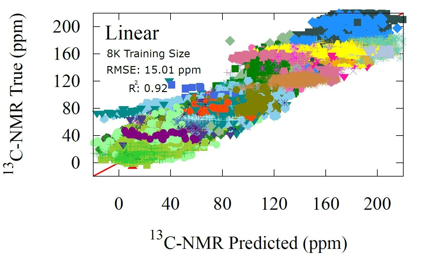

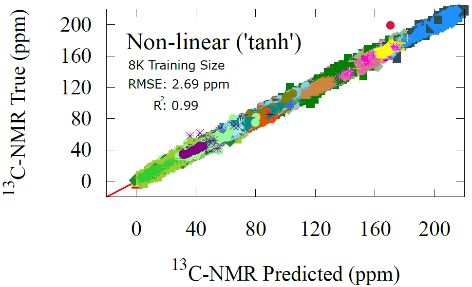
Fig 7 - NMR prediction performance of the non-linear transfer learning model trained on 8K datapoints. The non-linear model trained with 481 points achieved same precision as the linear, signifying a data limitation not an architectural one.
Fig 5 - three models used for transfer learning. 1) Linear regression (not shown) 2) 1-layer dense neural net, equation shown above with a diagram of the network architecture and 3) size-extensive neural net which employs model 2) in an extensive way to involve all atoms in molecules
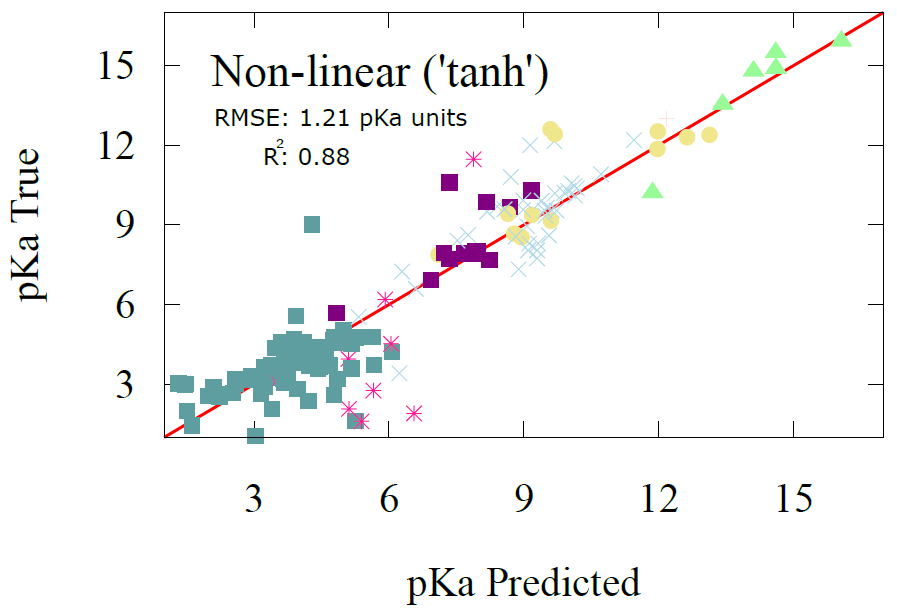
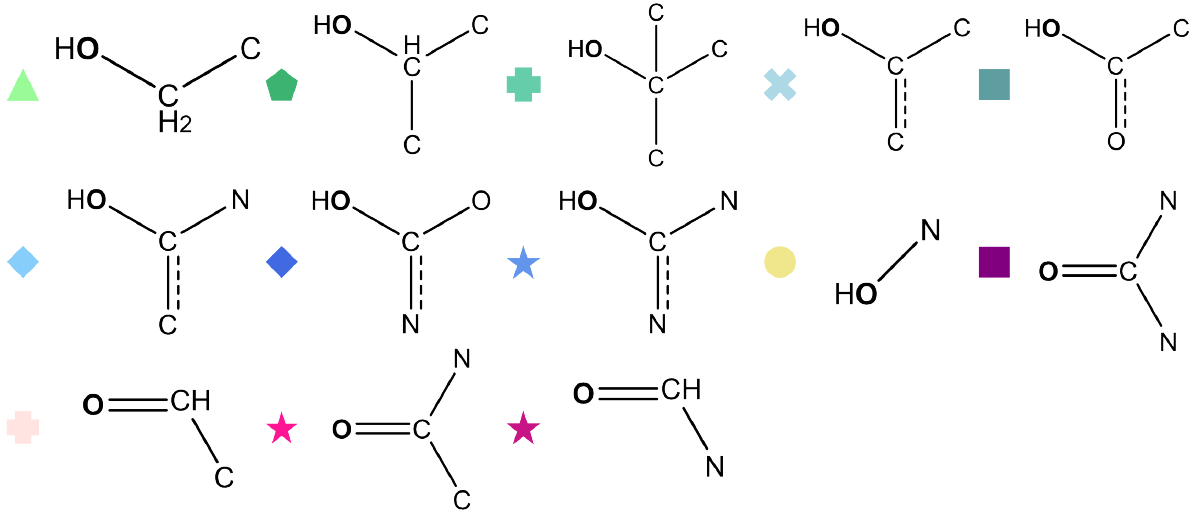
Fig 6 - performance of non-linear regression model on pKa dataset training on only 400 datapoints from IUPAC pKa. Results are shown for the 100 data point test set
C-NMR Transfer Learning Results
NMR is a site-specific electromagnetic property of molecles, when under magnetic field, nuclear spin is split into energy levels, one that aligns and one that misalignes with the field. This energy split is affected by the electrons shileding the nuclei and can be a great indicator the molecular structure around the atom, chemists use it widely to determine molecular structure.
For C-NMR prediction we evaluated four downstream models: a linear regression and a one layer neural network, each trained on two datasets of very different sizes and origins. The smaller dataset (NMRShiftDB2) contains experimental structures paired with NMR shifts generated by a structural fingerprinting method. The larger dataset (QM9NMR) provides DFT computed shifts for 10,000 molecules. Using both allows us to examine how transfer learning performance scales with data quantity.
For the small dataset, the linear regression achieves an RMSE of 15.01 ppm with a correlation coefficient of 0.92, which is already strong performance given that only 481 training points were available. The non linear model improves this only slightly, to 14.62 ppm and a correlation of 0.93. These results show that with limited data the AFV representation already contains most of the usable information and both models approach the same ceiling.
The picture changes when larger training sets are used. With 8000 points from QM9NMR, the linear model remains stuck near 15 ppm, unable to leverage the additional data. With just one layer of non-linearity in the second model, however, reduces the RMSE dramatically to 2.69 ppm. An error of 15 ppm. is qualitatively reasonable, but 2.69 ppm is within the accuracy range of high level methods such as DFT and close to state of the art GNN models. For reference, Han et al. achieved 2.38 ppm RMSE using hundreds of thousands of training examples. Our results show that the AFV representation allows a simple one layer network to approach this level of accuracy with an order of magnitude less data.
These results also illustrate a key limitation of small-dataset learning. With only a few hundred datapoints, the model cannot capture the full complexity of the AFV to property mapping, so both the linear and non-linear models converge to the same performance ceiling, regardless of how structured or expressive the AFV representation is. This explains why the linear model does not improve with more data, whereas the non-linear model improves dramatically once additional samples are available. In this regime the model is limited not by architecture or representation granularity but by the amount of signal present in the data itself. We can diagnose how much information is still missing by observing model behavior as dataset size grows. If the linear model saturates while the non-linear model continues to improve, this indicates that non-linear structure remains in the AFV space and that the dataset has not yet sampled that structure sufficiently.
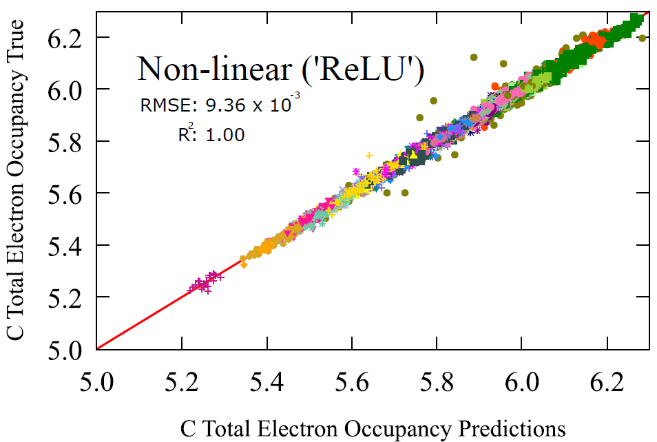
Fig 8 - Transfer learning performance on carbon occupancy with linear and non-linear regression.
Solubility Transfer Learning: A Molecule-Wide Property
As a final example, we consider a size extensive property, one that depends on the entire molecule rather than a specific atomic site. For this task we use the size-extensive model, which is the same one layer neural network described earlier, except now it is applied to every atom in the molecule. The atomwise outputs are then summed to produce the total solubility, which serves as the training target.
Solubility is an intrinsically complex property, influenced by thermodynamics, molecular polarity, hydrogen bonding, and the subtle interactions that arise when a solute becomes fully surrounded by water molecules. The quantity we predict is logS, the logarithm of the number of grams of solute that dissolve in a liter of water. Using only 640 training points from the NP MRD database, the model achieves competitive accuracy on a 160 point test set. The resulting RMSE OF 0.64 lies within the range of established physics based methods such as DFT and continuum solvation models, which typically achieve errors of roughly 0.5 to 2.0 units.
One challenge with size extensive models is interpreting the contribution that each atom makes to the total property. For solubility, such decomposition is not uniquely defined because solubility is a global thermodynamic quantity. Nevertheless, the atomwise contributions learned by the model can reveal useful patterns. To illustrate this, we plot the carbon centered contributions to logS against the first principal component of the AFV space, which captures broad structural differences between molecular environments (see previous post). Clear trends emerge. Carbons in hydrophobic environments, lacking nearby heteroatoms, contribute negatively to solubility, whereas carbons adjacent to oxygen or nitrogen tend to contribute positively. These trends reflect the chemical intuition underlying solubility and demonstrate that the AFV based size extensive model can learn interpretable structure property relationships from relatively small datasets.
More subtle trends also emerge from the atomwise contributions. The model identifies molecular symmetry as a factor that lowers solubility by canceling out local polarity. Several substituted carbon environments that appear hydrophilic at first glance — such as di nitrogen, tri nitrogen, di oxygen, tri carbon, or tetra carbon substituted carbons — display reduced solubility contributions once symmetry is considered. An interesting exception is tri oxygen substitution, which does not follow this pattern. In this case the third oxygen is typically part of a carbonyl group that breaks symmetry, whereas the di oxygen substitution remains symmetric. This suggests that the AFV representation continues to encode symmetry related information learned during GNN pretraining.
There are also counterintuitive trends that the model captures correctly. Simple methyl groups often contribute positively to solubility in small molecules, because their protrusion can disrupt symmetry and induce a weak net polarity. In contrast, O-methyl groups contribute negatively, despite breaking symmetry. This aligns with chemical intuition: an O-methyl substituent blocks a potential hydrogen bonding site, reducing the molecule’s ability to interact favorably with water. The AFV-based model recovers these subtle effects without explicit chemical rules, indicating that the learned representations retain nuanced information about symmetry, polarity, and local electronic environments.
Conclusions
Our results demonstrate that once a high-quality atom feature vector (AFV) space is learned via a pretrained GNN, even simple downstream models—linear regression or shallow neural networks—can achieve high accuracy on diverse chemical properties using only limited data. This shows that the core message-passing representation captures deep chemical structure in a transferable, property-agnostic latent space. The ability to recover site-specific properties (like pKa or NMR) and molecule-wide properties (like solubility or electron density) underscores the generality of the approach. Looking ahead, this paradigm opens the door to a new generation of data-efficient, interpretable models: once we build a robust chemical embedding space, we can rapidly adapt it for any new property — even with small experimental datasets — closing the gap between machine learning and practical chemistry.
References
For those interested in diving deeper into the details, all connecting citations and results discussed in this post can be found in our full article: [1] A. M. El-Samman, S. De Castro, B. Morton and S. De Baerdemacker. Transfer learning graph representations of molecules for pKa, 13C-NMR, and solubility. Canadian Journal of Chemistry, 2023, 102, 4.